Now that we have explored how to create maps and to download and plot occurrence data from the Paleobiology Database using R, let’s take a look at how to create paleogeographic maps.
Paleogeographic maps are reconstructions of the Earth’s surface at different points in geological time, showing the distribution of landmasses, oceans, and other features. GPlates is a program that enables users to model different geologic variables, including plate tectonics, into present and past maps. GPlates has a web service that provides access to various paleogeographic reconstructions that can be used in R. The first step is to download the data using a function from the sf package called st_read(). In this example, we will download a database of the coastlines (which can be used to reconstruct the continents) during the Late Cretaceous, more precisely, from 72 million years ago, using and plot it using the terra package. Such reconstructions are based on paleogeographical models and, in this example, we are going to specify the GOLONKA model, based on the Wright et al. 2013 publication.
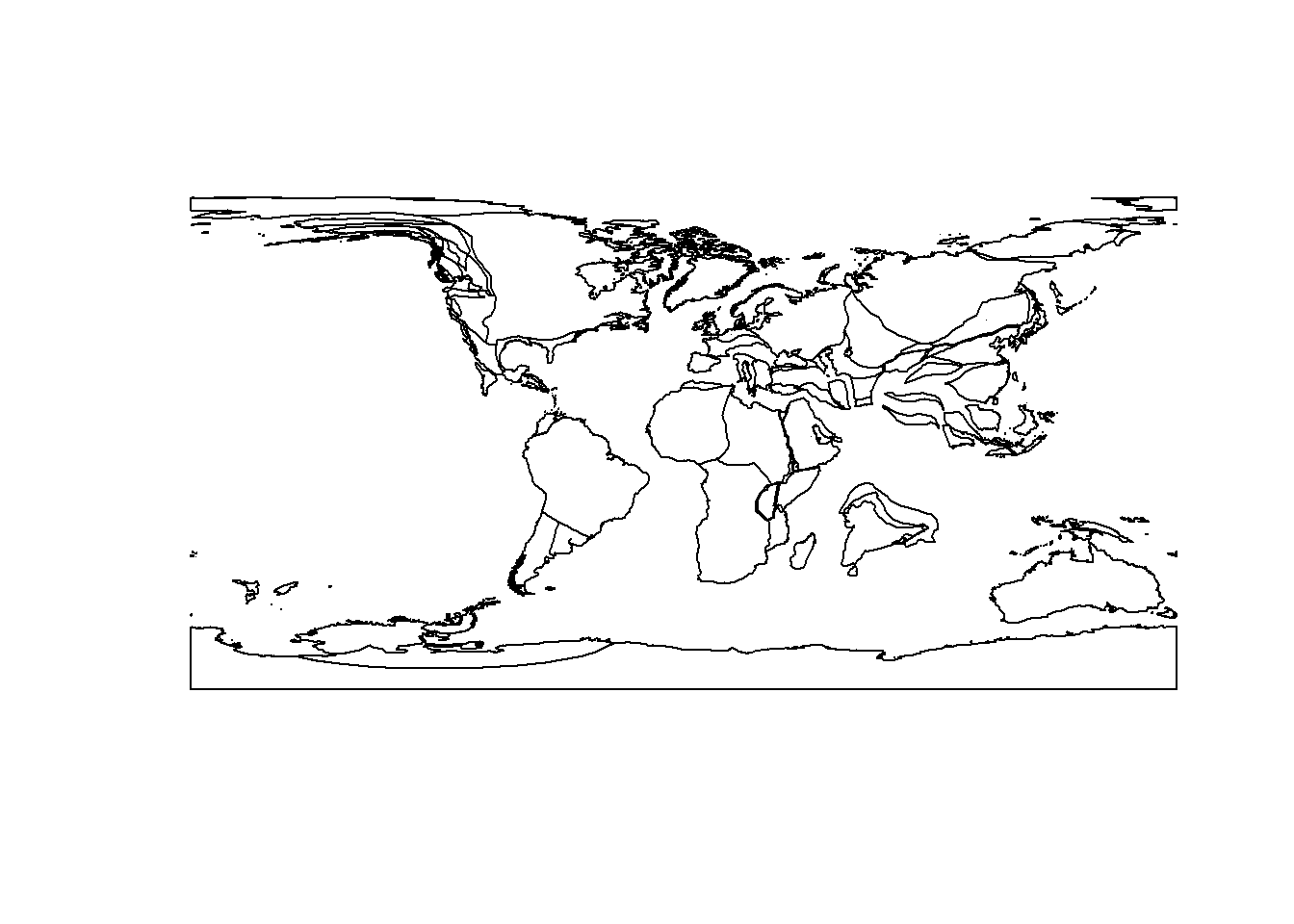
# first define an object containing the URL of the reconstructionpaleocoastlines.url <-"http://gws.gplates.org/reconstruct/coastlines/?time=72&model=GOLONKA"# then use st_read() to download itpaleocoastlines <-st_read(paleocoastlines.url)# simple plot to check itplot(paleocoastlines)
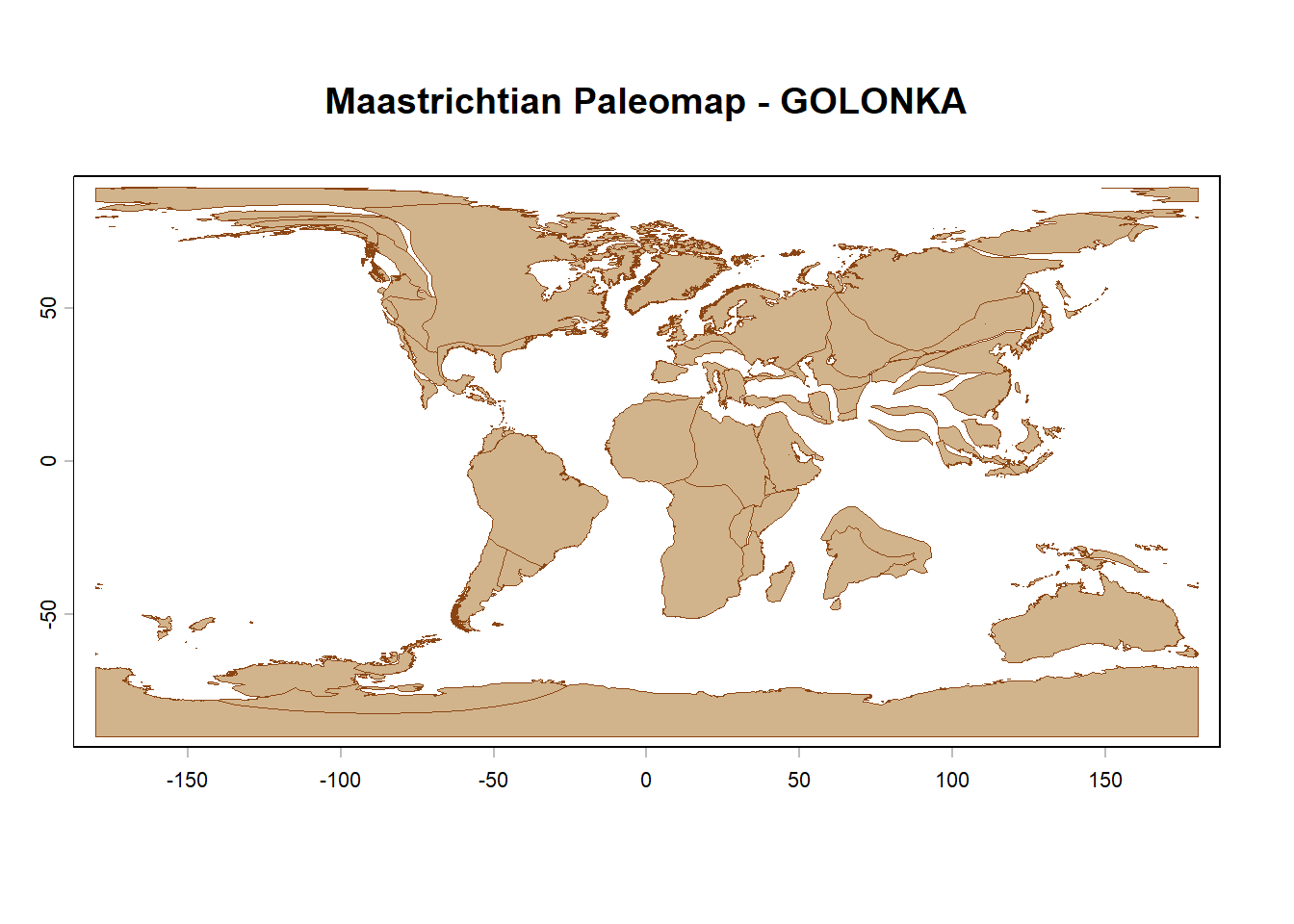
The object paleocoastlines is a simple features (sf) object that can be converted to a SpatVector object from the terra package using the function vect(). This allows us to use the plotting capabilities of the terra package to create more customized maps, such as adding colors and changing the borders’ width. Let’s convert the object and plot it using terra:
# convert to SpatVectorpaleocoastlines.terra <-vect(paleocoastlines)# plot using terraplot(paleocoastlines.terra,col ="tan",border ="saddlebrown",lwd =0.5,main ="Maastrichtian Paleomap - GOLONKA")
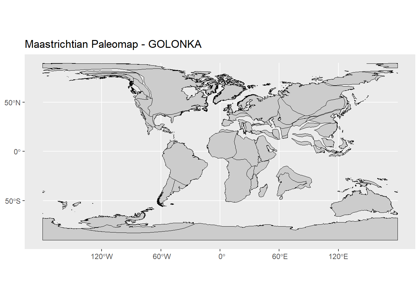
We can also use the original sf object to create maps using the ggplot2 package. This allows us to take advantage of the powerful plotting capabilities of ggplot2 to create more complex and visually appealing maps. Let’s see how to do that:
library(ggplot2)ggplot() +geom_sf(data = paleocoastlines, fill ="grey80", color ="black") +labs(title ="Maastrichtian Paleomap - GOLONKA")
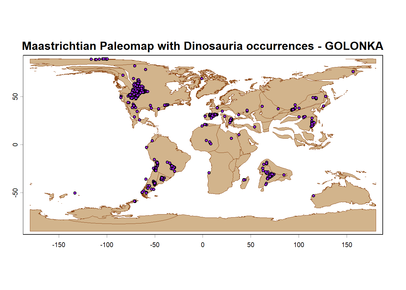
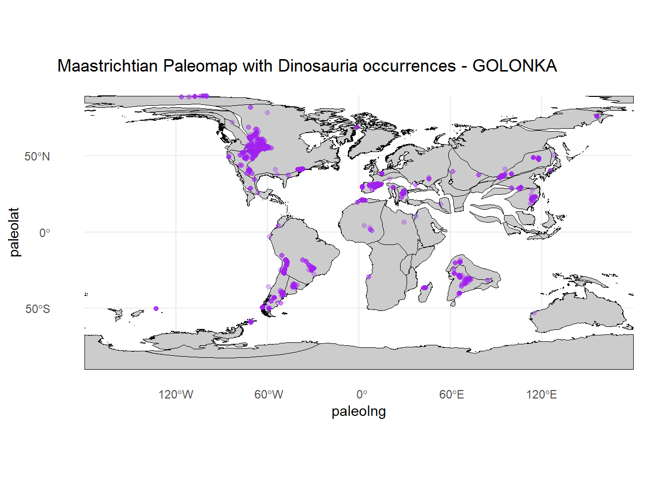
And, finally, we can of course add occurrence data to our paleogeographic maps. However, it is important to note that the coordinates of the occurrences need to be “paleoreconstructed” to match the time period of the paleomap. This can be done using various methods, such as using plate tectonic models or software like GPlates. Once the coordinates are reconstructed, we can plot them on top of the paleogeographic map using either terra or ggplot2.
library(paleobioDB)# download Dinosauria occurrences from the Maastrichtiandinosaurs.maastr <-pbdb_occurrences(base_name ="Dinosauria",interval ="Maastrichtian",show =c("coords", "classext", "paleoloc"),limit ="all", vocab ="pbdb",pgm ="gplates")# plot using terraplot(paleocoastlines.terra,col ="tan",border ="saddlebrown",lwd =0.5,main ="Maastrichtian Paleomap with Dinosauria occurrences - GOLONKA")points(dinosaurs.maastr$paleolng, dinosaurs.maastr$paleolat,pch =21,bg ="purple",cex =0.7)
# plot using ggplot2ggplot() +geom_sf(data = paleocoastlines, fill ="grey80", color ="black") +labs(title ="Maastrichtian Paleomap with Dinosauria occurrences - GOLONKA")+theme_minimal() +geom_point(data = dinosaurs.maastr,aes(x = paleolng, y = paleolat),colour ="purple",alpha =0.3,show.legend =FALSE)