Correlation is a statistical measure that can be used to test and describe the extent to which two continuous variables change together. It quantifies the strength and direction of the linear relationship between the variables. The correlation coefficient, often denoted as “r”, ranges from -1 to +1. A value of +1 indicates a perfect positive correlation, meaning that as one variable increases, the other variable also increases proportionally. A value of -1 indicates a perfect negative correlation, meaning that as one variable increases, the other variable decreases proportionally. A value of 0 indicates no correlation, meaning there is no linear relationship between the variables.
Correlation is defined in terms of the variance of x, the variance of y, and the covariance of x and y, that is, the way they vary together. The formula to obtain the correlation between x and y is the covariance between x and y, divided by the square root of the variance of x times the variance of y:
Let’s check whether there is a correlation between the SCL and SCm variables in the Ferreira et al. (2024) dataset. We will need to remove any observations containing NAs in either variable before checking for correlation.
# keep only the rows with complete cases for both SCm and SCLSCm.SCL <- F24.size[complete.cases(F24.size$SCm, F24.size$SCL), c("SCm", "SCL", "Clade")]attach(SCm.SCL)# calculate covariance between SCm and SCLcov(SCm, SCL)
[1] 4036.496
# calculate variance of SCm and SCL (separately)var(SCm)
[1] 842.2108
var(SCL)
[1] 24748.29
# calculate the correlation coefficient using the formulacorrelation_coefficient <-cov(SCm, SCL) /sqrt(var(SCm) *var(SCL))correlation_coefficient
[1] 0.8841411
There is of course a function to calculate the correlation coefficient implemented in the stats R package, which is cor(). Let’s confirm the results are the same as using the formula above:
cor(SCm, SCL)
[1] 0.8841411
Finally, it is also possible to statistically test for a correlation between two variables and to determine the significance of such correlation. This can be done using the cor.test() function. Check the help page for more details on how to use this function, particularly regarding the different methods available (Pearson, Spearman, Kendall) and for using more complex formulas. Here we will use the default method (Pearson):
cor.test(SCm, SCL)
    Pearson's product-moment correlation

data:  SCm and SCL
t = 29.861, df = 249, p-value < 2.2e-16
alternative hypothesis: true correlation is not equal to 0
95 percent confidence interval:
 0.8537893 0.9085031
sample estimates:
      cor
0.8841411
The output of the cor.test() function provides several pieces of information, including the correlation coefficient, the p-value, and the confidence interval for the correlation coefficient. A low p-value (less than 0.05) indicates that the correlation is statistically significant.
Regression
Regression is a statistical method used to examine the relationship between a dependent (response) variable and one or more independent (explanatory) variables, when they are both continues. It helps us understand how changes in the independent variables are associated with changes in the dependent variable. There are different types of regression, including linear regression, multiple regression, and logistic regression, each suited for different types of data and research questions. Here we will cover only linear regressions, which is the simplest and most frequently used type.
The basic function of regressions analyses is to estimate parameter values and their standard errors using the data available. The first step is to select a model to describe the relationship between the dependent and independent variables. The most common model is the linear model, which assumes a straight-line relationship between the variables. The general equation for a simple linear regression is:
y = a + bx where y is the dependent variable, a is the intercept (the value of y when x is 0), b is the slope (the change in y for a one-unit change in x), and x is the independent variable.
To perform a linear regression in R, we can use the lm() function. Let’s use the SCm as the dependent variable and SCL as the independent variable from the Ferreira et al. (2024) dataset and use the function summary() to view the results of the regression analysis:
linear_model <-lm(SCm ~ SCL, data = SCm.SCL)summary(linear_model)
Call:
lm(formula = SCm ~ SCL, data = SCm.SCL)

Residuals:
    Min      1Q  Median      3Q     Max
-59.497  -6.389  -1.774   4.701  67.568

Coefficients:
            Estimate Std. Error t value Pr(>|t|)
(Intercept) 1.891870   1.697558   1.114    0.266
SCL         0.163102   0.005462  29.861   <2e-16 ***
---
Signif. codes:  0 '***' 0.001 '**' 0.01 '*' 0.05 '.' 0.1 ' ' 1

Residual standard error: 13.59 on 249 degrees of freedom
Multiple R-squared:  0.7817,    Adjusted R-squared:  0.7808
F-statistic: 891.7 on 1 and 249 DF,  p-value: < 2.2e-16
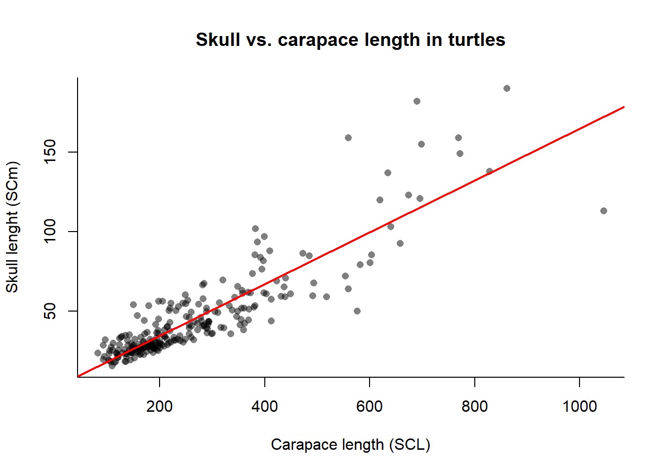
The output of the summary() function provides several pieces of information, including the coefficients (intercept and slope), their standard errors, t-values, and p-values. The R-squared value indicates the proportion of variance in the dependent variable that can be explained by the independent variable. To visualize the regression line along with the data points, we can use the plot() function to create a scatter plot and then add the regression line using the abline() function:
plot(x = SCL,y = SCm,main ="Skull vs. carapace length in turtles",xlab ="Carapace length (SCL)",ylab ="Skull lenght (SCm)", bty ="l",pch =16,col =rgb(0,0,0,0.5))# add the regression lineabline(linear_model, col ="red", lwd =2)
Regression formulas can also be used to predict values of y based on new values of x. For example, let’s predict the value of SCm when SCL = 645 using the stats function predict():
# create a data frame with the new value of SCLnew.SCm =data.frame(SCL =645)pred <-predict(linear_model, newdata = new.SCm, interval ="confidence")pred
       fit      lwr      upr
1 107.0927 102.7015 111.4839
The output provides the predicted value of SCm along with the lower and upper bounds of the confidence interval (defined with the argument interval of the predict() function) for the prediction.