There are different ways of selecting colors for plots in R. So far, we’ve seen the simplest way — but also the most limited — of selecting colors by using their names (e.g., “red”, “blue”, “green”, etc.). R has a set of predefined color names that you can use in your plots. You can see the full list of color names by running the colors() function:
head(colors(), n =20) ## show first 20 color names
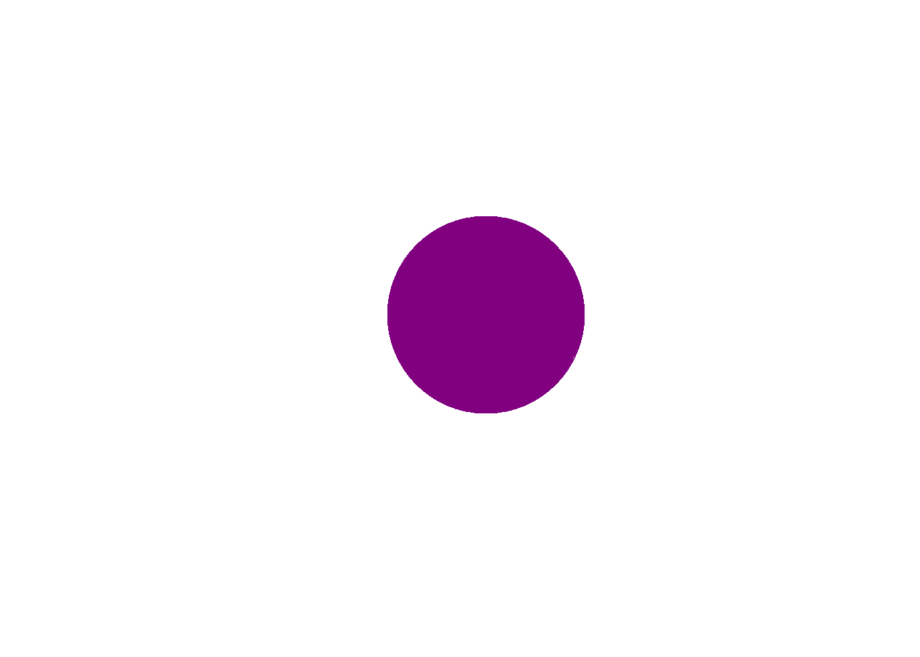
The rgb() function allows you to create custom colors by specifying the red, green, and blue components of the color. Each component can take a value between 0 and 255. For example, to create a custom purple color, you can use:`
plot(1, 1, col = custom.purple, pch =19, cex =20,xaxt ='n', ## removes x axisyaxt ='n', ## removes y axisxlab ="",ylab ="",bty ="n") ## removes box around the plot
You can also create colors using hexadecimal color codes. A hexadecimal color code is a six-digit code that represents the red, green, and blue components of a color. For example, the hexadecimal color code for pink is “#ff00ff”. You can use this code directly in your plots:
Another way to select colors is by using the hsv() function, which allows you to create colors based on their hue, saturation, and value (brightness). The hue component represents the color itself, the saturation component represents the intensity of the color, and the value component represents the brightness of the color. Each component can take a value between 0 and 1. For example, to create a custom orange color, you can use:
custom.orange <-hsv(h =30/360, s =1, v =1)custom.orange
Another nice feature is adding transparency to colors using the adjustcolor() function. This function allows you to adjust the transparency of a color by specifying an alpha value between 0 (completely transparent) and 1 (completely opaque). For example, to create a semi-transparent red color, you can use:
for (i in1:3) {plot(1, 1,col = colors.vector[i],pch =19,cex =20,xaxt ='n',yaxt ='n',xlab ="",ylab ="",bty ="n")}
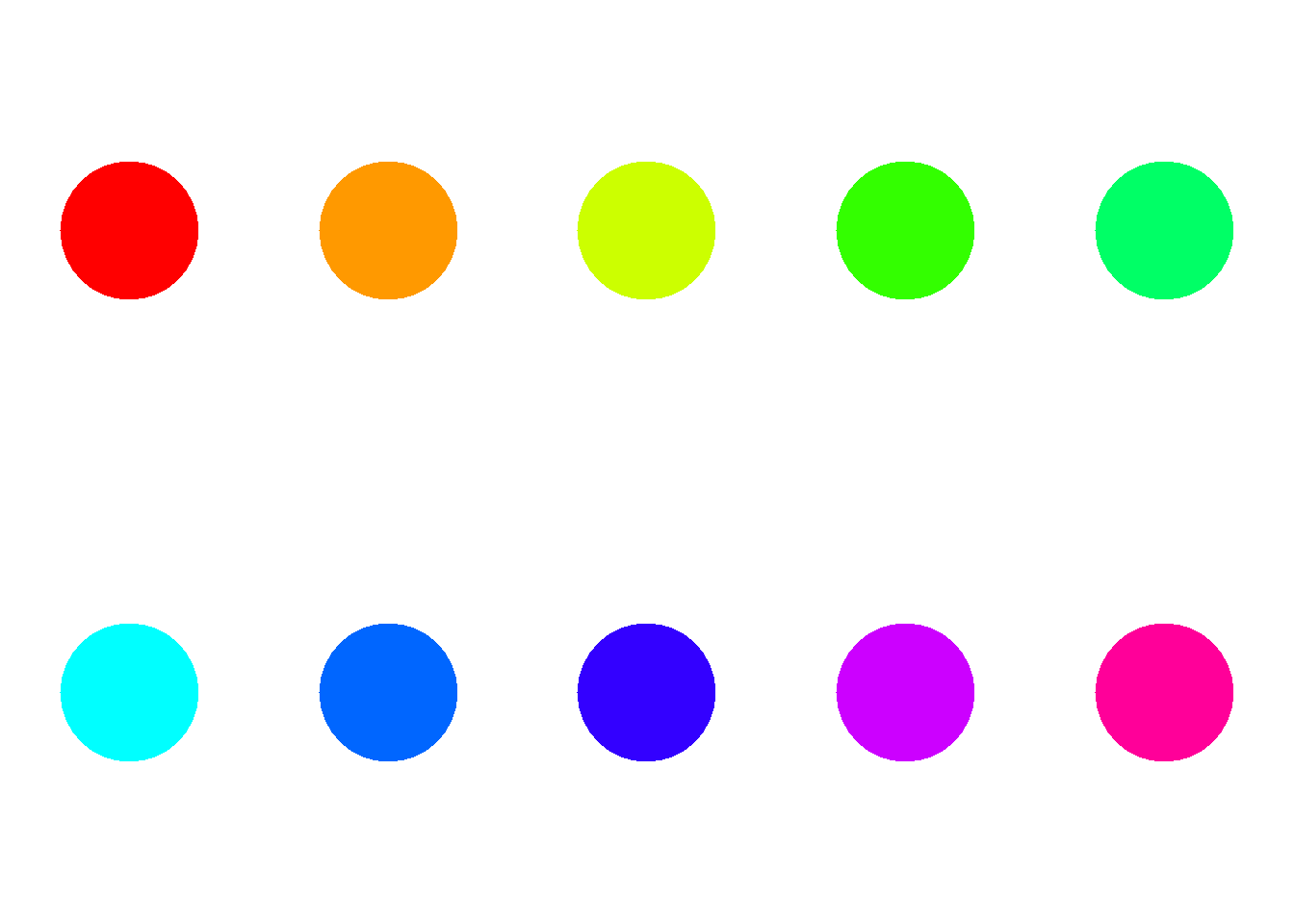
You can also use built-in color palettes in R, such as the rainbow(), heat.colors(), terrain.colors(), and topo.colors() functions. These functions generate a sequence of colors based on a specific color scheme. For example, to create a rainbow color palette with 10 colors, you can use:
rainbow.colors <-rainbow(10)par(mfrow =c(2,5), mai =c(0.3,0.3,0.3,0.3)) for (i in1:10) {plot(1, 1,col = rainbow.colors[i],pch =19,cex =15,xaxt ='n',yaxt ='n',xlab ="",ylab ="",bty ="n")}
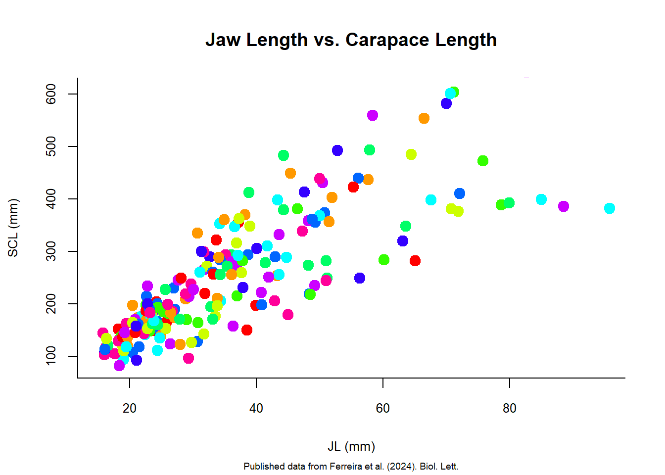
You can use these colors in your plots by specifying them in the col argument. For example, let’s create a scatter plot using the rainbow color palette:
setwd("d:/R Projects/Intro-to-R/datasets/Ferreira_etal-2024")size.meas <-read.csv("size-meas.csv", sep =",", header =TRUE)plot(size.meas$JL, size.meas$SCL,xlim =c(15,95), ylim =c(80,610),xlab ="JL (mm)",ylab ="SCL (mm)",main ="Jaw Length vs. Carapace Length",sub ="Published data from Ferreira et al. (2024). Biol. Lett.",bty ="l",col = rainbow.colors,pch =19,cex =1.5,cex.main =1.2,cex.sub =0.6,cex.lab =0.8,cex.axis =0.8)
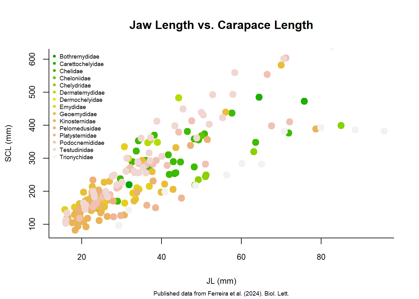
In this example, the colors are assigned based on the order of the points in the dataset (i.e., row 1 gets position one in rainbow.colors object, row 2 gets position 2 and so on). You can customize the color assignment based on your specific needs. For example, you can assign colors based on a categorical variable in your dataset, such as the Clade of the turtles. This way, each clade will have a different color in the plot. Here is an example using the terrain.colors pallete:
clade.colors <-terrain.colors(length(unique(size.meas$Clade)))names(clade.colors) <-unique(size.meas$Clade)point.colors <- clade.colors[size.meas$Clade]plot(size.meas$JL, size.meas$SCL,xlim =c(15,95), ylim =c(80,610),xlab ="JL (mm)",ylab ="SCL (mm)",main ="Jaw Length vs. Carapace Length",sub ="Published data from Ferreira et al. (2024). Biol. Lett.",bty ="l",col = point.colors,pch =19,cex =1.5,cex.main =1.2,cex.sub =0.6,cex.lab =0.8,cex.axis =0.8)legend("topleft", legend =names(clade.colors), col = clade.colors, pch =19, cex =0.6,bty ="n")